Fundamentals
- Initializing
- Getting
- Setting
- Slicing
a = np.array([1, 2, 3, 4, 5, 6])
a
---------------
array([1, 2, 3, 4, 5, 6])


a[0]
---------------
1

a[0] = 10
a
---------------
array([10,  2,  3,  4,  5,  6])

a[:3]
---------------
array([10, 2, 3])
Accessing Values Note
It is familiar practice in mathematics to refer to elements of a matrix by the row index first and the column index second. This happens to be true for two-dimensional arrays, but a better mental model is to think of the column index as coming last and the row index as second to last. This generalizes to arrays with any number of dimensions.
Creating Quick Arrays
| Code | Output |
|---|---|
np.zeros(2) | array([0., 0.]) |
np.ones(2) | array([1., 1.]) |
np.empty(2) | array([3.14, 42. ]) # may vary |
np.arange(4) | array([0, 1, 2, 3]) |
np.arange(2, 9, 2) | array([2, 4, 6, 8]) |
np.linspace(0, 10, num=5) | array([ 0. , 2.5, 5. , 7.5, 10. ]) |
x = np.ones(2, dtype=np.int64) | array([1, 1]) |
Basic Slicing and Getting
data = np.array([[1, 2], [3, 4], [5, 6]])
-> array([[1, 2],
       [3, 4],
       [5, 6]])

data[0, 1]
-> 2

data[1:3]
-> array([[3, 4],
       [5, 6]])

data[0:2, 0]
-> array([1, 3])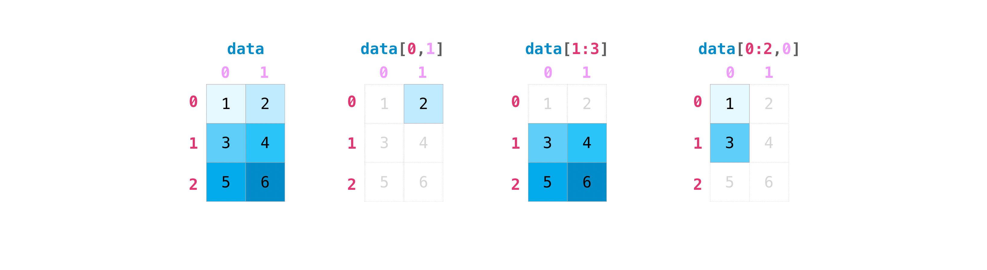
Bool Indexing
a[a < 5]: Returns all values in a less than 5- Literally the values:
[1 2 3 4]out of
np.array([[1 , 2, 3, 4], [5, 6, 7, 8], [9, 10, 11, 12]])
- Literally the values:
Shape
| Code | Output |
|---|---|
a = np.arange(6) | [0 1 2 3 4 5] |
b = a.reshape(3, 2) | [[0 1], [2 3], [4 5]] |
a1 = np.array([[1, 1],[2, 2]])a2 = np.array([[3, 3],[4, 4]]) | |
np.vstack((a1, a2)) | array([[1, 1],[2, 2],[3, 3],[4, 4]]) |
np.hstack((a1, a2)) | array([[1, 1, 3, 3],[2, 2, 4, 4]]) |
Numpy Views
By default, Numpy returns views (or literally a reference to a piece of the original array) to save memory, so if these are modified the original is modified as well.
This means that if something needs to be mutable, a copy should be created.
b = a.copy
Inbuilt operations
- Numpy supports array element per element operations
a + bwhere both are arrays, as well as-,*,/ - Supports quick sum of array
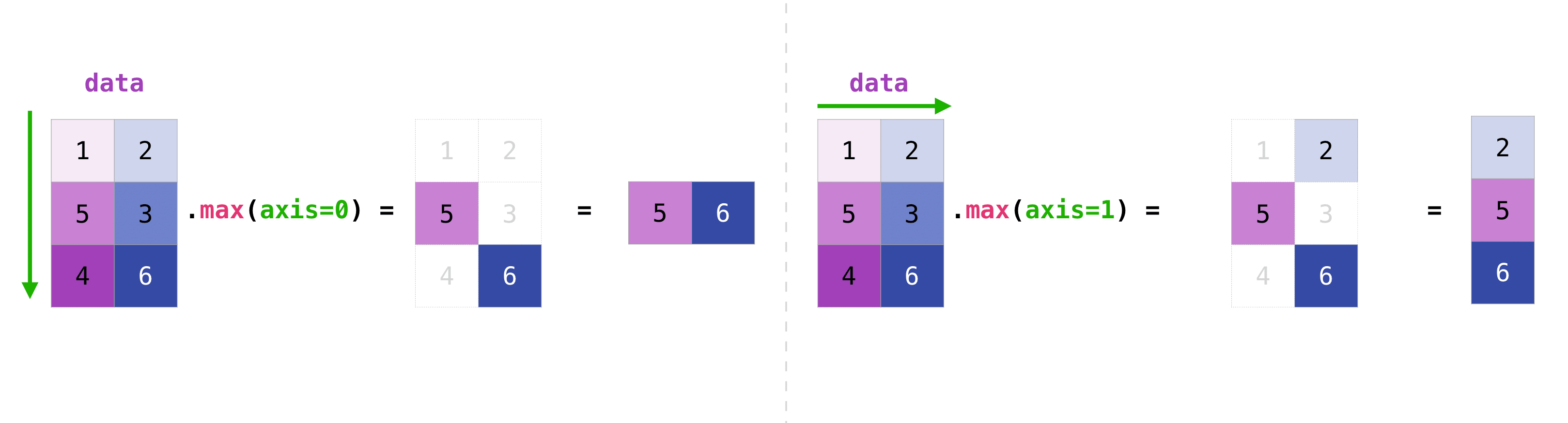
b = np.array([[1, 1], [2, 2]])
b.sum(axis=0) -> array([3, 3])
b.sum(axis=1) -> array([2, 4]) - Array times scalar
data = np.array([1.0, 2.0])
data * 1.6 -> array([1.6, 3.2]) - Useful operations:
min, max, sum, mean, prod (for multiplication), std, and more
Cleaning
a = np.array([11, 11, 12, 13, 14, 15, 16, 17, 12, 13, 11, 14, 18, 19, 20])

unique_values = np.unique(a)
unique_values -> [11 12 13 14 15 16 17 18 19 20]

unique_values, indices_list = np.unique(a, return_index=True)
indices_list -> [ 0  2  3  4  5  6  7 12 13 14]

unique_values, occurrence_count = np.unique(a, return_counts=True)
occurrence_count -> [3 2 2 2 1 1 1 1 1 1]
Can reverse an array with rev = np.flip(arr)
- Can flip 1D, 2D, or nested arrays.
Flattening arrays
Flattening creates a copy, ravel creates a reference
x = np.array([[1 , 2, 3, 4], [5, 6, 7, 8], [9, 10, 11, 12]])

x.flatten()
-> array([ 1,  2,  3,  4,  5,  6,  7,  8,  9, 10, 11, 12])

a2 = x.ravel()
a2[0] = 98 -> [98  2  3  4  5  6  7  8  9 10 11 12]
print(x) -> [[98  2  3  4]
			 [ 5  6  7  8]
			 [ 9 10 11 12]]
Saving
You can save Numpy array’s to disk with load, save, and savez
np.save('filename', a)-> Save a singly ndarray objectb = np.load('filename.npy')
Linear Algebra
Matrices are represented by 2d numpy.array objects.
Can use the @ operator for computing matrix product.
Many more functions that I don’t recognize (Einstein summation, Kronecker product), come back later as necessary
| Code | Function |
|---|---|
numpy.dot(a,b) | Dot product of two arrays, returns output |
.vdot(a, b) | Return the dot product of two vectors. |
.inner / .outer (a,b) | Computes inner and outer product respectively |
.linalg.matrix_power(a, n) | Raise a square matrix to the (integer) power n. |
.linalg.cross | Returns the cross product of 3-element vectors. |
.linalg.svd (a, full_matrices=True, compute_uv=True, hermitian=False) | Singular Value Decomposition |
.linalg.svdvals (x, /) | Returns the singular values of a matrix (or a stack of matrices) x. |
.linalg.eig (a) | Compute the eigenvalues and right eigenvectors of a square array. (eigh to calculate for a complex Hermitian or a real symmetric matrix) |
.linalg.eigvals (a) | Compute the eigenvalues of a general matrix. (same as above, can extend with h) |
| Can also calculate: |
norm, condition number, determinant, matrix rank, trace
Can solve equations and invert matrices
Also support Fourier Transform
The library supports a Fast Fourier Transform (FFT)
However,
The SciPy module scipy.fft is a more comprehensive superset of numpy.fft, which includes only a basic set of routines.
ChatGPT
Overview
NumPy (Numerical Python) is a fundamental library for numerical computations in Python. It provides support for large, multi-dimensional arrays and matrices, along with a collection of mathematical functions to operate on these arrays.
Key Features
- Efficient array operations
- Mathematical and statistical functions
- Linear algebra, Fourier transforms, and random number generation
- Integration with other libraries like SciPy and Pandas
Core Data Structures
- ndarray: The central data structure in NumPy, a multi-dimensional array object that is faster and more compact than Python’s built-in lists.
Important Functions and Methods
Array Creation
np.array(object, dtype=None): Create an array from any object exposing the array interface.np.zeros(shape, dtype=float): Create an array of zeros with the specified shape and type.np.ones(shape, dtype=float): Create an array of ones with the specified shape and type.np.arange(start, stop, step, dtype=None): Create an array with evenly spaced values within a given interval.np.linspace(start, stop, num=50, endpoint=True): Create an array with evenly spaced values over a specified interval.
Array Operations
array.shape: Returns the dimensions of the array.array.reshape(new_shape): Reshape the array without changing its data.array.flatten(): Flatten a multi-dimensional array into a 1D array.np.concatenate((a1, a2, ...), axis=0): Join a sequence of arrays along an existing axis.np.split(array, indices_or_sections, axis=0): Split an array into multiple sub-arrays.
Mathematical Functions
np.add(x1, x2): Element-wise addition.np.subtract(x1, x2): Element-wise subtraction.np.multiply(x1, x2): Element-wise multiplication.np.divide(x1, x2): Element-wise division.np.dot(a, b): Dot product of two arrays.np.sum(array, axis=None): Sum of array elements over a specified axis.np.mean(array, axis=None): Mean of array elements over a specified axis.np.std(array, axis=None): Standard deviation of array elements over a specified axis.
Linear Algebra
np.linalg.inv(a): Compute the (multiplicative) inverse of a matrix.np.linalg.eig(a): Compute the eigenvalues and right eigenvectors of a square array.np.linalg.svd(a): Singular Value Decomposition.
Random Number Generation
np.random.rand(d0, d1, ..., dn): Generate random values in a given shape.np.random.randint(low, high=None, size=None): Return random integers fromlow(inclusive) tohigh(exclusive).np.random.normal(loc=0.0, scale=1.0, size=None): Draw samples from a normal (Gaussian) distribution.
Documentation & Resources
- Official NumPy Documentation
- NumPy GitHub Repository
- NumPy Tutorials & Examples
- NumPy Cheat Sheet
Common Use Cases
- Array operations and manipulations
- Mathematical computations and linear algebra
- Random number generation for simulations
- Integration with data analysis libraries like Pandas and SciPy
Example Code
import numpy as np

# Creating arrays
arr1 = np.array([1, 2, 3, 4])
arr2 = np.array([[1, 2], [3, 4]])

# Array operations
print("Array 1:", arr1)
print("Array 2:\n", arr2)

# Reshaping and concatenation
arr3 = arr1.reshape((2, 2))
print("\nReshaped Array:\n", arr3)
arr4 = np.concatenate((arr2, arr3), axis=0)
print("\nConcatenated Array:\n", arr4)

# Mathematical operations
sum_arr = np.add(arr1, arr1)
print("\nSum of Array 1 with itself:", sum_arr)

# Linear algebra
matrix = np.array([[1, 2], [3, 4]])
inverse_matrix = np.linalg.inv(matrix)
print("\nInverse of Matrix:\n", inverse_matrix)