📗 -> 10/1/24:
🎤 Vocab
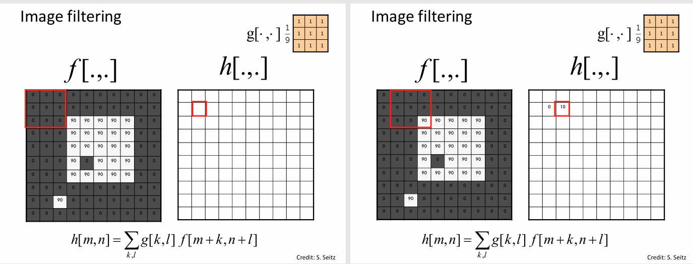
Convolution - The averaging of a pixel with the pixels surrounding it. A graphic of the process is shown below
- Results in a ‘smoothing’ effect
Convolution is a more general and powerful technique that uses a kernel (a small matrix) to scan an image, element-wise multiplying each pixel value with the corresponding kernel element
❗ Unit and Larger Context
Final Project
40 Points
• Big Project– Better if related to your own research
• Proposal is due on 4/30/2023 at 11:59pm
– Less than a page
– The problem that you want to solve
– Motivation: why is this an important problem to solve.
– What dataset you will use.
– What method you will use to solve it.
– Crisp final outcome/deliverable
• Final report, code, and presentation video due on 6/7/2023 at 11:59pm
✒️ -> Scratch Notes
A pixel in 2D space mapping to a brightness:
Image operations:
- Map an image onto a greyscale version of the image:
- Transform the image, maybe remove the background
- Turn the image into a vector of values (maybe a float representing brightness)
- Compare similarity of two images
Getting Rid of Noise:
Convolution is very helpful. This is an example of a box filter. Multiplying by a matrix with an ‘eye’ (3x3 where all values are zero except for (2,2)=1) outputs the same image.
Different types of filters:
Smoothing:
A box filter similar to above.
Sharpening:
Multiply with a matrix with a eye greater than 1. Increasing all values.
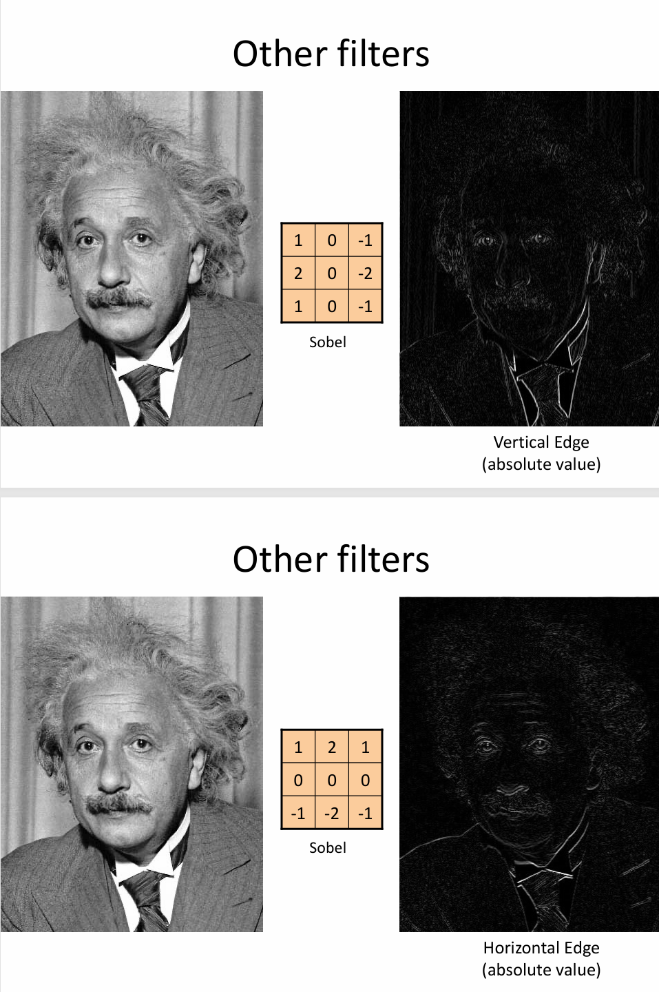
Edge Detection:
A Sobel kernel, accentuates edges
Horizontal kernel: [-1 0 1; -2 0 2; -1 0 1]
Vertical kernel: [-1 -2 -1; 0 0 0; 1 2 1]
Gradient Filter:
Horizontal Gradient: [-1, 0, 1]
Vertical Gradient: [-1; 0; 1]
Gaussian:
You can convolve an image with a Gaussian matrix, where the center is more heavily weighted than outsides, according to the Gaussian equation
- Gaussian filters are softer than box filters. Box filters often create artifacts.
- Variance of the Gaussian determines the extent of smoothing.
- Parameter
is the “scale” / “width” / “spread” of the Gaussian kernel, and controls the amount of smoothing. - Z is normalizing to 1, making it so that the area under the curve sums to 1
Combining Filters:
Filters are associative
This can be particularly useful in a Gaussian blur, where the horizontal and vertical blurs combine to give a 2D Gaussian blur, while being a much faster operation
The Gaussian is separable
Left operation is much slower than right, while being equivalent
Not all filter are separable
🧪-> Example
- List examples of where entry contents can fit in a larger context
🔗 -> Related Word
- Link all related words